This guide explains equilibrium pricing for leaders in manufacturing and distribution, including pricing, revenue, and finance. It covers the definition, calculation methods, and practical steps to implement equilibrium pricing as a discipline to protect margins.
What Is Equilibrium Pricing?
The equilibrium price is the price at which the quantity buyers demand equals the quantity sellers supply. At that price, the market clears. As N. Gregory Mankiw defines it in Principles of Economics (9th edition, 2023), it is the point where “supply and demand are in balance.”
While this definition is suitable for introductory economics, B2B pricing is more complex. Industrial and distribution markets often involve unequal bargaining power, contract variability, and changing capacity constraints. For operators, equilibrium pricing is not a single value but a range within which the firm can clear capacity at an acceptable margin, given real competitive and cost conditions.
Key Distinctions
Equilibrium price versus equilibrium quantity: P* represents the per-unit price, while Q* is the volume transacted at that price. In B2B settings, pricing is often determined by a known-quantity target, such as capacity or a sales plan. This reversal is significant.
Market-clearing versus optimal price: A market-clearing price clears the market, while a profit-maximizing price focuses on maximizing contribution margin. This may involve leaving some capacity unused if higher margins on fewer units improve overall profitability. Confusing these concepts is a common mistake in applied pricing.
Related terms: Price elasticity of demand measures how quantity responds to price changes. In B2B, demand is often inelastic, with research showing industrial elasticities as low as −0.03 to −0.40. This suggests many firms have more pricing flexibility than they realize. Willingness to pay (WTP) is the maximum a customer is willing to pay, typically estimated by segment to move from a single price to a profitable price corridor. Net price realization, the actual revenue collected per unit after all discounts, rebates, and deductions, connects equilibrium theory to financial outcomes.
Why Equilibrium Pricing Matters in B2B
The difference between current B2B pricing and the true equilibrium range leads to margin loss. This issue, known as pricing drift, is the gradual and often unnoticed erosion of net price realization due to unmonitored discounting, outdated cost-plus practices, and a lack of price governance.
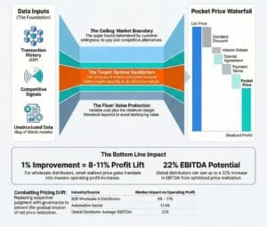
The financial evidence is clear. A McKinsey analysis of the S&P 1500 found that a 1% improvement in price yields an average 8% increase in operating profit. A more recent McKinsey study of 130 global distributors put that figure at 22% of EBITDA. Yet the 2024 Simon-Kucher Global Pricing Study (n = 2,704) found only 65% of firms possess genuine pricing power, and by 2025, average price realization had fallen to just 43% — down five percentage points in two years. Separately, Bain reports that 85% of B2B executives believe their pricing decisions need improvement.
Without an equilibrium anchor, discount approvals become arbitrary, pricing reviews rely on subjective judgment, and margin erosion accumulates over time.
The Equilibrium Pricing Model
The classical model uses downward-sloping demand and upward-sloping supply curves that intersect at equilibrium. In B2B practice, these curves are rarely visible. Instead, firms rely on transaction data, reflecting actual prices paid by specific customers in particular channels and timeframes.
A practical approach is to ask: At what price does the firm fill its target capacity while achieving the highest possible contribution margin? This integrates demand sensitivity, cost structure, and capacity utilization into one operational framework.
How to Calculate Equilibrium Price
Algebraic Method
For linear demand, set quantity demanded equal to quantity supplied and solve for price. If demand is Q(P) = a − bP and supply is fixed at capacity C, then P* = (a − C) / b. This method is useful for quick estimates, though real markets are often more complex.
Graphical Method
Plot the estimated demand against your supply constraint and identify the intersection point. This approach is useful in pricing workshops to build intuition before using statistical models. Analyzing historical discount curves can provide an empirical demand curve.
Statistical / Causal Estimation
For serious pricing operations, equilibrium estimation requires econometric demand modeling. A causal approach — such as Double Machine Learning (DML) — isolates the true price-quantity relationship from confounders like seasonality, promotions, and competitive activity. Research by Bajari et al. (2015, NBER) demonstrated that ML methods produce more accurate out-of-sample demand predictions than traditional approaches, particularly in high-dimensional B2B environments.

Data Inputs You Need
Required data falls into five categories: (1) Transaction history, including invoice-level data with actual prices, quantities, customer identifiers, and dates, covering at least 18–24 months. (2) Cost data at the SKU or product-family level. (3) Capacity and supply constraints, such as production limits, inventory, and lead times. (4) Competitive pricing signals, including price indices, win/loss data, and public price lists. (5) Market and segment variables, such as geography, contract type, order size, seasonality, and demand drivers. Clean, detailed transaction data is the most critical input. Data preparation often requires more time than modeling, especially when reconstructing price waterfalls from complex ERP systems.
Estimating Your Equilibrium Price Range
In practice, equilibrium pricing works best as a price corridor with three boundaries:
Floor — variable cost plus minimum margin threshold. Below this, every incremental unit destroys value. Target — the price at which estimated demand equals target capacity utilization at an attractive contribution margin. Ceiling — the upper bound set by WTP, competitive alternatives, and price sensitivity.

This corridor approach recognizes that customers in different segments have varying price sensitivities. Effective pricing and revenue management programs establish corridors at the segment or product-family level and enforce them through discount approval rules and deal desk governance.
Worked Example: B2B Distributor Equilibrium Calculation
A mid-market industrial distributor: 10,000 units monthly capacity, $72 variable cost per unit, estimated demand Q(P) = 16,000 − 50P, target minimum contribution margin of 35%.
Step 1: Capacity-clearing price. 10,000 = 16,000 − 50P → P* = $120.
Step 2: Margin check. CM = $120 − $72 = $48 per unit (40%). Exceeds the 35% target.
Step 3: Total contribution. 10,000 × $48 = $480,000/month.
Step 4: Build the corridor. Floor: $72 ÷ 0.65 ≈ $112 (minimum acceptable). Target: $120. Ceiling: $130 (at $130, demand = 9,500 units, still 95% utilization).
Step 5: Validate using elasticity. E = (−50)(120/10,000) = −0.60. Demand is inelastic at this price, indicating potential to increase prices for segments with lower sensitivity.
How Organizations Apply Equilibrium Pricing: Three Examples
Managing capacity constraints via price corridors. A global data storage and electronics manufacturer faced cyclical markets where demand for high-capacity enterprise products routinely outstripped supply. They implemented an allocation committee workflow backed by analytics: when supply was the binding constraint, pricing logic shifted from maximizing volume to maximizing margin. A revenue and profit decomposition module separated changes into new business, lost business, and existing business — revealing whether price increases caused genuine demand destruction or merely shed unprofitable customers. Elasticity modeling identified the floor price (the point where further discounting degraded margin without generating incremental lift), establishing the bottom of their corridor.
Establishing equilibrium in competitive, unregulated markets. A multinational pharmaceutical company selling branded generics in emerging markets faced aggressive local competitors. Their static pricing frequently left them either too high (losing volume) or too low (leaving margin on the table). The team built a Product Equivalence Matrix mapping their SKUs to competitor SKUs, then set Competitive Price Index (CPI) corridors by brand tier — for example, a “Premium” brand targeted 110–120% of the average generic price. Products dipping below 110% were flagged as underpriced; those exceeding 120% risked volume collapse. Dashboard alerts let local teams adjust list prices in near real time to recapture their equilibrium position.
Navigating cost-push inflation without destroying demand. A national beverage manufacturer needed to pass rising input costs through to retailers without triggering delisting. They deployed a Price-Volume-Mix decomposition that isolated how much of their revenue change was driven by price realization versus cost inflation, then used scenario planning to simulate the new equilibrium: “How much volume will we lose if we cover the full cost increase?” The analysis surfaced a critical constraint most pricing teams miss — retailer velocity hurdles. If a price increase pushed demand below the retailer’s minimum velocity threshold, the product would be pulled from shelves. The pricing strategy was calibrated to keep velocity above that threshold while still recovering cost inflation.

KPIs to Monitor Around Your Equilibrium Price
Five metrics tell you whether your organization is operating within its corridor:
Net price realization — actual collected price divided by list price. Track weekly by segment. If it trends below your floor, pricing drift is active.
Pocket margin — revenue minus all variable costs and off-invoice deductions. The true economic margin after the entire price waterfall has been applied.
Win rate by price band — track at the floor, target, and ceiling. Stable win rates as you move toward the ceiling suggest a conservatively set corridor.
Competitive price index (CPI) — your price relative to the benchmark. A CPI between 95 and 105 typically indicates you are near market equilibrium.
Discount exception rate — deals approved below the floor. Healthy is under 10%. Above 20%, your governance has become a rubber stamp.
Common Pitfalls
Treating equilibrium as a fixed number. It varies by segment, geography, channel, and time. Build segment-specific corridors, not national averages.
Assuming equilibrium equals profit-maximizing price. In capacity-constrained environments, the profit-maximizing price often sits above the market-clearing price. Always model contribution margin, not just volume clearance.
Using the historical average price as a proxy. Your historical average reflects past discounting behavior, which McKinsey research indicates was too low in 80–90% of cases. It perpetuates underpricing rather than diagnosing it.
Skipping the market boundary definition. Equilibrium is meaningless without a defined scope: products, segments, geography, and time window.
Ignoring the regulatory dimension. The FTC’s revival of Robinson-Patman Act enforcement (FTC v. Southern Glazer’s, December 2024; FTC v. PepsiCo, January 2025) means differential pricing now requires documented economic justification. Segment-level equilibrium pricing must be supported by cost-to-serve analysis and formalized pricing governance.
Implementation Roadmap: 30–90 Days
Days 1–30: Diagnose. Reconstruct your price waterfall to pocket margin. Quantify the gap between the list and actual net price realization. Identify the three to five largest leakage sources. Stand up a dashboard with the five KPIs above. Form a cross-functional pricing team.
Days 31–60: Build corridors. Estimate demand curves for top product families. Set corridors by segment. Design deal desk rules: auto-approve within the corridor, escalate below the floor with documented justification. Pilot in one region or product line.
Days 61–90: Operationalize. Roll out corridors across the first wave of products. Monitor net price realization and discount exception rates daily. Establish a monthly pricing committee to review corridor performance, approve exceptions, and recalibrate as market conditions shift. Begin sales enablement on value selling within the corridor.

Operationalizing Equilibrium Pricing
The key difference between companies that achieve their equilibrium range and those that do not is governance, not analytics. Three elements are essential: decision rights (clearly define who approves pricing at each threshold, such as auto-approval for discounts under 5%, manager sign-off for 5–15%, and director or VP approval with rationale for above 15%); guardrails (set corridor limits in quoting tools so that pricing outside the corridor requires a deliberate override); and cadence (establish monthly reviews, quarterly recalibration, and annual resets).
A balanced pricing approach combines equilibrium corridors with rule-based automation. In practice, rule-based systems that enforce corridor boundaries and flag exceptions capture most of the value of dynamic pricing, while minimizing complexity and organizational resistance.
FAQ: Equilibrium Pricing
What is meant by equilibrium pricing? It is the process of identifying and setting prices at or near the point where demand equals available supply. In B2B, it means finding the price range where your firm fills target capacity at an acceptable margin, then governing decisions to stay within that range.
What is an example of an equilibrium price? In the worked example above, a distributor with 10,000 units of monthly capacity and demand Q(P) = 16,000 − 50P arrives at an equilibrium price of $120, where demand exactly matches capacity at a 40% contribution margin.
What is an equilibrium pricing model? A model combining demand estimation with supply or capacity constraints to identify the market-clearing price. It can range from algebraic calculation to causal econometric models that account for confounders and segment heterogeneity.
What is the equilibrium price strategy? Using data on demand, costs, and capacity to establish a defensible price corridor (floor, target, ceiling) by segment, then enforcing that corridor through deal desk governance and performance monitoring.
What is the equilibrium price in one word? Balance.
How do you calculate the equilibrium price? Set quantity demanded equal to quantity supplied and solve for price. For Q(P) = a − bP with fixed supply C: P* = (a − C) / b. In practice, estimate the demand function from transaction data using regression or causal ML methods.
Is equilibrium pricing the same as profit-maximizing pricing? No. Equilibrium clears the market; profit-maximizing pricing maximizes contribution margin, which may mean selling fewer units at higher margins, especially in capacity-constrained settings.
Does equilibrium pricing mean matching competitors? No. It accounts for competitive dynamics as one input, but is anchored in your own costs, capacity, demand curve, and segment economics. A differentiated firm may have an equilibrium well above its competitors.
What to Do Next
The difference between current pricing and data-driven equilibrium is measurable and often represents several percentage points of operating margin. Addressing this gap begins with diagnosing the current state, estimating the equilibrium range, and establishing governance to maintain it.
For a structured starting point, Revology Analytics provides a pricing and revenue management diagnostic. This service assesses your current price waterfall, estimates equilibrium ranges for your top product families, and identifies the fastest paths to margin recovery, typically delivering measurable financial impact within 90–120 days.